A clue to duality

High energy physics researchers still rely on the concept that it is the nucleus of the photon that they must isolate in order to measure (observe) the particle.

The nucleus is only a “concentration” of “some” of the energy.
When this concentration becomes enough to be detected,  it has already  formed a stable structure complete with polarity and field lines.
The particle’s field lines are comprised of “the same” energy; only smaller… As is the nucleus.

If you are looking for the nucleus of a photon, you immediately run into a problem. Your assumption asserts that the photon’s existence is contained within it’s nucleus. It is not.
A piece of energy, or a particle is comprised of many smaller, individual, pieces of the same energy. The nucleus is only a concentration of the energy, and is only “part” of the atomic structure of the photon.

All interaction, with any part of this structure, will cause interference, if forced into a frame of reference. Since the photon is a “sum of it’s parts,” any attempt (accidental or otherwise) to reference just the nucleus will fail, and any point that is detected will reference the entire piece of energy as if it were in that location.

The only “assertion” David has really made.

…”But we must realize that the fields around an electron, as well as all around

other matter are actually two opposing bowl shaped electromagnetic fields.

Unless we properly understand this basic magnetic field structure,

we will never be able to properly understand the fundamental forces of matter

from the sub-atomic to the galactic.”   David LaPoint

Baffling pulsar leaves astronomers in the dark

http://sci.esa.int/xmm-newton/51314-baffling-pulsar-leaves-astronomers-in-the-dark/

24 January 2013

New observations of a highly variable pulsar using ESA’s XMM-Newton are perplexing astronomers. Monitoring this pulsar simultaneously in X-rays and radio waves, astronomers have revealed that this source, whose radio emission is known to ‘switch on and off’ periodically, exhibits the same behaviour, but in reverse, when observed at X-ray wavelengths. It is the first time that a switching X-ray emission has been detected from a pulsar, and the properties of this emission are unexpectedly puzzling. As no current model is able to explain this switching behaviour, which occurs within only a few seconds, these observations have reopened the debate about the physical mechanisms powering the emission from pulsars.

Artist’s impression of a pulsar in radio-bright mode. Credit: ESA/ATG medialab

Few classes of astronomical objects are as baffling as pulsars – which were discovered as flickering sources of radio waves and soon after interpreted as rapidly rotating and strongly magnetised neutron stars. Even though about 2000 pulsars have been found since the first was discovered in 1967, a detailed understanding of the mechanisms that power them still eludes astronomers.

“There is a general agreement about the origin of the radio emission from pulsars: it is caused by highly energetic electrons, positrons and ions moving along the field lines of the pulsar’s magnetic field, and we see it pulsate because the rotation and magnetic axes are misaligned,” explains Wim Hermsen from SRON, the Netherlands Institute for Space Research in Utrecht, The Netherlands. “How exactly the particles are stripped off the neutron star’s surface and accelerated to such high energy, however, is still largely unclear,” he adds.

Hermsen led a new study based on observations of the pulsar known as PSR B0943+10, which were performed simultaneously in X-rays, with ESA’s XMM-Newton, and in radio waves. By probing the emission from the pulsar at different wavelengths, the study had been designed to discern which of various possible physical processes take place in the vicinity of the magnetic poles of pulsars. Instead of narrowing down the possible mechanisms suggested by theory, however, the results of Hermsen’s observing campaign challenge all existing models for pulsar emission, reopening the question of how these intriguing sources are powered.

“Many pulsars have a rather erratic behaviour: in the space of a few seconds, their emission becomes weaker or even disappears for a while, just to go back to the previous level after some hours,” says Hermsen. “We do not know what causes such a switch, but the fact that the pulsar keeps memory of its previous state and goes back to it suggests that it must be something fundamental.”

Recent studies indicate that the switch between what are usually referred to as ‘radio-bright’ and ‘radio-quiet’ states is correlated to the pulsar’s dynamics. As pulsars rotate, their spinning period slows down gradually, and in some cases the slow-down process has been observed to accelerate and slow down again, in conjunction with the pulsar switching between radio-bright and quiet states. The existence of correlated variations in both the rotation and emission suggest a connection between a pulsar’s immediate vicinity and, on a grander scale, its co-rotating magnetosphere, which may extend up to about 50 000 km for objects like PSR B0943+10. In order for the radio emission to vary so radically on the short timescales observed, the pulsar’s global environment must undergo a very rapid – and reversible – transformation.

“Since the switch between a pulsar’s bright and quiet states links phenomena that occur on local and global scales, a thorough understanding of this process could clarify several aspects of pulsar physics. Unfortunately, we have not yet been able to explain it,” says Hermsen.

Artist’s impression of a pulsar in X-ray-bright/radio-quiet mode. Credit: ESA/ATG medialab

Hermsen and his colleagues planned to search for an analogous pattern at a different wavelength – in X-rays – to investigate what causes this switching behaviour. They chose as their subject PSR B0943+10, a pulsar that is well known for its switching behaviour at radio wavelengths and for its X-ray emission, which is brighter than might be expected for its age.

“Young pulsars shine brightly in X-rays because the surface of the neutron star is still very hot. But PSR B0943+10 is five million years old, which is relatively old for a pulsar: the neutron star’s surface has cooled down by then,” explains Hermsen.

Astronomers know of only a handful of old pulsars that shine in X-rays and believe that this emission comes from the magnetic poles – the sites on the neutron star’s surface where the acceleration of charged particles is triggered. “We think that, from the polar caps, accelerated particles either move outwards to the magnetosphere, where they produce radio emission, or inwards, bombarding the polar caps and creating X-ray emitting hot-spots,” Hermsen adds.

There are two main models that describe these processes, depending on whether the electric and magnetic fields at play allow charged particles to escape freely from the neutron star’s surface. In both cases, it is believed that the emission of X-rays follows that of radio waves, but the emission that is observed in each scenario is characterised by different temporal and spectral characteristics. Monitoring the pulsar in X-rays and radio waves at the same time, the astronomers hoped to be able to discern between the two models.

Obtaining observing time on the requested telescopes turned out to be a rather lengthy procedure. “We needed very long observations, to be sure that we would record the pulsar switching back and forth between bright and quiet states several times,” says Hermsen, “So we asked for a total of 36 hours of observation with XMM-Newton. This is quite a lot of time, and it took us five years before our proposal was accepted.”

The two states of pulsar PSR B0943+10 as observed with XMM-Newton and LOFAR. Credit: ESA/ATG medialab; ESA/XMM-Newton; ASTRON/LOFAR

The observations were performed in late 2011. The X-ray monitoring performed with XMM-Newton was accompanied by simultaneous observations at radio waves from the Giant Metrewave Radio Telescope (GMRT) in India and the recently inaugurated Low Frequency Array (LOFAR) in the Netherlands, which was used during its commissioning phase, while testing its science operations.

“The X-ray emission of pulsar PSR B0943+10 beautifully mirrors the switches that are seen at radio wavelengths but, to our surprise, the correlation between these two emissions appears to be inverse: when the source is at its brightest in radio waves, it reaches its faintest in X-rays, and vice versa,” says Hermsen.

The XMM-Newton data also show that the source pulsates in X-rays only during the X-ray-bright phase – which corresponds to the quiet state at radio wavelengths. During this phase, the X-ray emission appears to be the sum of two components: a pulsating component consisting of thermal X-rays, which is seen to switch off during the X-ray-quiet phase, and a persistent one consisting of non-thermal X-rays. Neither of the leading models for pulsar emission predicts such behaviour.

“The data collected during our monitoring campaign are truly challenging our understanding of pulsars, since no current model is able to explain them,” comments Hermsen. “In the second half of 2013, we plan to repeat the same study for another pulsar, PSR B1822-09, which exhibits similar radio emission properties, but is characterised by a different geometrical configuration. This will allow us to study these extreme objects under different viewing angles,” he adds.

In the meantime, these observations will keep theoretical astrophysicists busy investigating possible physical mechanisms that could cause the sudden and drastic changes to the pulsar’s entire magnetosphere and result in such a curious emission.

“The unpredictable behaviour of this pulsar, revealed using the great sensitivity of the telescopes on board XMM-Newton, may require a radically new approach to study the fundamental processes that power these fascinating objects,” comments Norbert Schartel, XMM-Newton Project Scientist at ESA.

Notes for editors

The study presented here is based on X-ray observations of pulsar PSR B0943+10 performed with ESA’s XMM-Newton between 4 November and 4 December 2011. These observations consisted of six observations in the energy range between 0.2 and 10 keV, each lasting six hours. The X-ray data were gathered at the same time as observations at radio wavelengths performed with the Indian Giant Metrewave Radio Telescope (GMRT) at 320 MHz and the international Low Frequency Array (LOFAR) at 140 MHz.

The research was led by Wim Hermsen (SRON Netherlands Institute for Space Research and Astronomical Institute ‘Anton Pannekoek’, University of Amsterdam), Lucien Kuiper and Jelle de Plaa (SRON Netherlands Institute for Space Research), Jason Hessels and Joeri van Leeuwen (ASTRON and Astronomical Institute ‘Anton Pannekoek’, University of Amsterdam), Dipanjan Mitra and Rahul Basu (NCFRA-TIFR, Pune, India), Joanna Rankin (University of Vermont, Burlington, USA), Ben Stappers (University of Manchester, UK), and Geoffrey Wright (University of Sussex, UK). The Pulsar Working Group and the Builders Group from the LOFAR-telescope, which was at the time in the commissioning phase, supported the observations.

The European Space Agency’s X-ray Multi-Mirror Mission, XMM-Newton, was launched in December 1999. It is the biggest scientific satellite to have been built in Europe and uses over 170 wafer-thin cylindrical mirrors spread over three high throughput X-ray telescopes. Its mirrors are among the most powerful ever developed. XMM-Newton’s orbit takes it almost a third of the way to the Moon, allowing for long, uninterrupted views of celestial objects. The scientific community can apply for observing time on XMM-Newton on a competitive basis.

Related publications

W. Hermsen, et al., “Synchronous X-ray and Radio Mode Switches: a Rapid Global Transformation of the Pulsar Magnetosphere“, 2013, Science, 339, 6118, 436-439, DOI:10.1126/science.1230960

Contacts

Wim Hermsen
SRON Netherlands Institute for Space Research
Utrecht, The Netherlands
and Astronomical Institute ‘Anton Pannekoek’
University of Amsterdam, The Netherlands
Email: w.hermsensron.nl
Phone: +31-88-7775871; +31-614547929

Norbert Schartel
ESA XMM-Newton Project Scientist
Directorate of Science and Robotic Exploration
European Space Agency
Email: Norbert.Schartelesa.int
Phone: +34-91-8131-184

http://phys.org/news/2013-01-chameleon-pulsar-baffles-astronomers.html

America’s Next Era in Space. The Plasma Universe

Einstein On The Porch:

It’s Sunday or so says the calendar and the habit of knowing what day it is because it tells me what my responsibilities are, or should be, is waning as a natural consequence of fully immersing myself in the Florida environment I have contemplated for 20 years or so.

The calendar may be the first to go into obsolescence followed shortly afterward by my watch thus allowing my full perception of the time-space continuum in new contexts and my place in it.

The cranes now stroll to within 30-feet of my back porch and I don’t obstruct their movement with my movement for a camera or even a sip from my coffee cup because for a few minutes I am not a steward of nature but part of it.

The first day of my calculus class years ago the teaching assistant announced, Anything known to man can be expressed through math,” and as she walked through the aisles of desks gifting us with the course syllabus I waited for her arrival.

When she handed me the paper I asked her, “How does math express beauty?”

She smiled and surely made a mental note she had a trouble maker in her class.

NASA Admits Alcubierre Drive Initiative: Faster Than The Speed Of Light

  

NASA is currently working on the first practical field test toward the possibility of faster than light travel.

 

Traveling faster than light has always been attributed to science fiction, but that all changed when Harold White and his team at NASA started to work on and tweak the Alcubierre Drive. Special relativity may hold true, but to travel faster or at the speed of light we might not need a craft that can travel at that speed. The solution might be to place a craft within a space that is moving faster than the speed of light! Therefore the craft itself does not have to travel at the speed of light from it’s own type of propulsion system.

 

It’s easier to think about if you think in terms of a flat escalator in an airport. The escalator moves faster than you are walking! In this case, the space encompassing the ship would be moving faster than the ship could fly, keeping all the matter of the ship intact. Therefore, we can move faster than light, in a massless cloud of space-time.

 

What is the Alcubierre Drive? It’s actually based on Einsteins field equations, it suggests that a spacecraft could achieve faster-than-light travel. Rather than exceed the speed of light alone in a craft, a spacecraft would leap long distances by contracting space in front of it and expanding space behind it. This would result in faster than light travel (1). Physicist Miguel Alcubierre was the first that we know to identify this possibility. He described it as remaining still on a flat piece of space-time inside a warp bubble that was made to move at “superluminal” (faster than light) velocity. We must not forget that space-time can be warped and distorted, it can be moved. But what about  moving sections of space-time that’s created by expanding space-time behind the ship, and by contracting space-time in front of the ship?

 

This type of concept was also recently illustrated by Mathematician James Hill and Barry Cox at the University of Adelaide. They published a paper in the journal proceedings of the Royal Society A: Mathematical and Physical Sciences (3).

 

It was once believed that Einsteins  theory of special relativity means that faster than light travel is just not possible. This is a misconception, special relativity simply states that the distance you travel depends on how fast you move, for how long you’re moving for. So if you are driving at 70 mph you will have covered 70 miles in one hour. The confusing part is that, no matter how fast you are moving you will always see the speed of light as being the same. It’s similar to sound, if you close your eyes and imagine that the only sense you have is hearing, you will identify things by how they sound. So if a car is driving at a rapid speed and honks its horn, we know that the horn is always tooting the same tone, it’s just the car’s motion that made it appear to change.

Special relativity also showed us that the atoms and molecules that make up matter are connected by electromagnetic fields, the same stuff light is made up of. The object that would break the light speed barrier is made up of the same stuff as the barrier itself. How can an object travel faster than that which links it’s atoms? This was the barrier.

 

The only problem with our modern day science is that creating distortions in space-time require energy densities that are not yet possible for humans, or so they say. NASA scientists are currently working on tweaking Alcubierre’s model.

 

Faster-than-light travel, also known as hyper space or “warp” drive from what the masses know for sure is currently at the level of speculation. Although there is already a lot of evidence that shows it is possible  and has already been accomplished, mainstream science is still catching up.  We are at the point right now where faster-than-light travel is still theoretical, but possible.

 

At the same time, we have to look at other factors that are now coming to light. As former NASA Astronaut and Princeton Physics Professor Dr, Brian O’leary Illustrates. This topic has recently had another media explosion and congress recently discussed and looked at evidence for Earth like planets recently found by Kepler Telescopes. Three “super-Earths” to be exact that are most probably teeming with life (4). Furthermore, former congressmen and women recently participated in a citizens hearing on the subject of UFOs a few weeks ago. You can read more about that here. I’ve used this video in many articles before, but it’s just a great clip from when Dr O’leary was still with us.

UFOs and the technology behind it should not be subject to speculation. Odds are we have retrieved some of that technology, or manufactured some ourselves. Some of our science may not be so theoretical after all.

 

“We now have the technology to take ET home” – Ben Rich

http://www.collective-evolution.com/2013/05/28/nasa-admits-they-are-working-to-travel-faster-than-the-speed-of-light/

 

Related articles

• Is Warp Drive Possible? (33rdsquare.com)

 

Demonstration of an inductively coupled ring trap for cold atoms

Abstract

We report the first demonstration of an inductively coupled magnetic ring trap for cold atoms. A uniform, ac magnetic field is used to induce current in a copper ring, which creates an opposing magnetic field that is time-averaged to produce a smooth cylindrically symmetric ring trap of radius 5 mm. We use a laser-cooled atomic sample to characterize the loading efficiency and adiabaticity of the magnetic potential, achieving a vacuum-limited lifetime in the trap. This technique is suitable for creating scalable toroidal waveguides for applications in matter-wave interferometry, offering long interaction times and large enclosed areas.

GENERAL SCIENTIFIC SUMMARY
Introduction and background. Trapping and manipulation of particles in a ring geometry is of interest on length scales varying from the giant LHC at CERN, to atoms trapped in microscopic optical vortices about the focus of laser beams. One particular advantage of a ring trap is its closed geometry, meaning that trapped particles are confined to a finite space but without any confinement in one dimension. The lack of azimuthal trapping is interesting, as this complete degree of freedom opens a one-dimensional phase space for exploration.

Main results. We have implemented a new type of ring trap for cold atoms that is conceptually different from existing technology. We utilize Faraday’s law to induce an alternating current in an isolated conducting loop of copper, through application of an external, time-varying magnetic field. The induced current in turn creates a spatially varying magnetic-field near the loop, which, when superimposed with the drive field, creates a magnetic minimum that traps ultra-cold atoms. Using induced current means that the undesired perturbations due to the magnetic-field from connecting wires are eliminated. We demonstrate that this technique can store atoms on second-long scales, limited by the background vacuum pressure.

Wider implications. Our results show a method of making toroidal traps that inherently minimize roughness of the potential. This geometry is being actively explored for atom interferometry with long interrogation times to develop precision rotation sensors, which could offer unprecedented sensitivity for internal navigation, reducing the dependence upon GPS.

1. Introduction

Development of ring traps for cold atoms is an active topic of theoretical and experimental study, motivated by the ability to create one-dimensional waveguides with periodic boundary conditions, which have applications in two regimes. For radii smaller than ~ 100 μm these traps can be filled with quantum degenerate gases, enabling studies of persistent current flow of a superfluid in a multiply connected geometry to realize atomtronic [1] analogues to a SQUID [2, 3] or of Hawking radiation from sonic black holes [4]. Alternatively, large radius rings can be utilized to create a matter-wave interferometer [5]. Atom interferometry is sensitive to both inertial effects and external fields and has been used to perform precision measurements of rotation [6–8], acceleration and gravitation [9, 10], in addition to determination of fundamental constants [11], magnetic gradients [12] and ac Stark shifts [13]. State-of-the-art experiments typically use unguided atoms, requiring large path lengths at which point acceleration due to gravity or the Coriolis force due to the Earth’s rotation becomes significant [14]. Ring traps provide an ideal geometry for these applications due to the common-mode rejection of the identical paths, with trivial extension of the enclosed area using multiple revolutions [8]. They are especially suited to performing rotation measurements using the Sagnac effect [15]. As the rotation sensitivity of a Sagnac interferometer is directly proportional to the enclosed area, large area interferometers are desirable [16].

Early techniques for generating large area ring waveguides exploited dc magnetic traps to create large ring [16, 17] and stadium [18] geometries. One of the challenges in producing scalable magnetic traps is avoiding losses from Majorana spin-flips at field zeros, which can be achieved using time-averaged magnetic fields [19, 20, 33] or radio-frequency (rf) dressing [21–24]. These methods can be combined to realize time-averaged adiabatic potentials [25, 26] to create versatile traps with adaptable radii. For studies of persistent flow in quantum fluids small traps with r ~ 20 μm are required which are possible using combined magnetic and optical or all optical traps [3, 27–29]. A novel technique to create time-averaged toroidal potentials using mechanical oscillation of a magnetic nanowire has recently been proposed [30].

In this paper, we demonstrate a large radius ring trap created from the time-averaged potential arising from the current induced in a conducting ring [31], suitable for applications in the regime of atom interferometry. A key benefit to this trapping scheme is that the geometry is defined by a macroscopic circular conductor, avoiding end effects associated with dc electromagnetic traps that act to break the cylindrical symmetry of the ring [32]. The other advantage is that the ac field averages out any roughness in the magnetic field to create a smooth trapping potential.

2. Theory

An inductively coupled ring trap for cold atoms is realized using the configuration shown schematically in figure 1(a), where a small conducting ring of radius r_ring is placed at the centre of two pairs of Helmholtz coils, one of which produces a time-varying ac drive field and another providing a uniform dc bias field both perpendicular to the plane of the ring. The time-varying magnetic field induces a current in the ring proportional to the rate of change of the magnetic flux through the ring, which following Griffin et al [31] is given by

where R and L are the electrical resistance and inductance of the ring, Ω = ωL/R is the ratio of the ac drive frequency to the natural low-pass frequency of the ring and δ₀ = tan⁻¹(1/Ω) is the phase-shift of the induced current. The current induced in the ring creates a spatially inhomogeneous magnetic field B_ring(r,z), as illustrated schematically in figure 1(c). Inside the ring this field opposes the drive field B₁(t) in figure 1(b) such that at any time in the cycle the total instantaneous magnetic field vanishes on a circle inside the ring radius, as indicated in figure 1(d).

Figure 1. Inductive ring trap. (a) A small copper ring is placed at the centre of two pairs of Helmholtz coils that provide an ac magnetic field at frequency ω (green coils) and a static bias field (grey coils) along the -axis. Gravity acts along . Panels (b)–(d) show the magnetic field along in the plane of the copper ring at time t = 0, where (b) is the ac drive field and (c) is the magnetic field created by the out of phase induced current in the ring. The total field is shown in (d), resulting in a field zero indicated by that is time-averaged to give a magnetic ring trap.

If the ac drive frequency ω is much larger than the frequency of atomic motion within the trap (typically  ~ 100 Hz for magnetic traps), the effective magnetic field experienced by an atom is given by the field magnitude averaged over one cycle  [19, 31, 33], where T = 2π/ω is the cycle period. The resulting time-averaged field magnitude creates a cylindrically symmetric trapping potential U = m_F g_F μ_B〈B〉 for atoms in weak-field-seeking states with m_F g_F  > 0 that provides both radial and axial confinement to create a toroidal trap. This is seen from figure 2(a) which plots 〈B〉 in the plane of the ring (z = 0) calculated for Ω = 20, with a steep barrier on the outside of the trap due to the large magnetic field close to the conducting ring and a parabolic local maximum at the origin. Minimization of 〈B〉 with respect to r shows the radius of the time-averaged minimum r_trap is located at the point where the inhomogeneous field of the ring is equal to . As the induced field B_ring∝B₀, the trap radius is determined purely by the conductor geometry. In addition, for Ω  1 the induced current is independent of resistance. Thus the trap radius is robust against fluctuations in the external field amplitude and the effects of Ohmic heating. The ac current also averages out corrugations caused by current meandering within the conductor [34, 35] to create a smooth, symmetric potential.

Figure 2. Time-averaged ring potential. (a) Cycle-averaged B-field magnitude in the plane of the ring creating an axially symmetric minimum inside the conductor radius. (b) Radius of the zeros in the instantaneous magnetic field during the ac cycle, calculated for Ω = 20 with no external bias (black) and for B_b = 0.1B₀ (red) to show the zeros being excluded from the trap centre at r/r_ring = 0.8 due to the bias field, preventing Majorana spin-flips. (c) Finite element simulation of the induced current density within the cross-section of the copper ring used in the experiment for B₀ = 110 G at ω/2π = 30 kHz, showing the current is strongly localized to the outer edge of the ring. (d) Time-averaged trapping potential for |F = 2,m_F  = + 2〉 state of Rb including gravity, calculated from the current distribution in (c) for B_b = 5 G. White circles indicate positions of field-zeros across the cycle, white cross indicates trap minimum and the black cross marks the saddle point used to define the trap depth.

 

In order for the atomic magnetic dipole to follow the external field adiabatically it is necessary for the Larmor frequency to be much larger than the rate of change of the magnetic field given by  [36]. If this condition is not met, then the atom can undergo a Majorana spin-flip into an un-trapped magnetic spin state and is lost from the ring. For the time-averaged potential it is the instantaneous value of the field, which must meet the adiabaticity criterion at all times in the cycle requiring |B(t)| > 0. Figure 2(b) plots the radial coordinate of the instantaneous zero r₀ throughout the cycle, which shows that the magnetic field zeros spend the majority of the time centred at the trap minimum r_trap, and sweep through the whole ring plane at times t = T/4 and 3T/4 due to the phase-lag between the driving and induced fields. Thus atoms loaded into the trap would be rapidly lost due to the non-adiabatic potential within a few cycles of the ac field. It is therefore necessary to apply an external dc bias field to move the field-zeros away from the trap minimum. The trivial solution is to place a current carrying wire aligned along the -axis through the centre of the ring to generate a radially symmetric azimuthal magnetic field [16]. However, this approach has a number of drawbacks as it compromises optical access within the ring trap and the end effects of the wire can break the symmetry. It also reduces the scalability of the ring trap for creating traps with radii of a few mm.

Instead we consider the case of a uniform dc bias field that is generated using a second pair of Helmholtz coils as shown in figure 1(a), which acts to offset the ac field to remove the field zeros. A lower limit for the bias required to remove the zeros from the trap centre can be obtained analytically from the amplitude of the combined ac field at r_trap using the relation for B_ring(r_trap,0) given above such that , which simplifies to

corresponding to 5.5 G for a 110 G drive field and Ω = 20. As the bias is increased, the circle of zero field is pushed out from the trap centre, creating inner and outer radii in the plane of the ring outside of which atoms are lost, analogous to the ‘circle of death’ in a TOP trap [33]. The effect of the bias field can be seen clearly from figure 2(b), where the zeros no longer sweep through the trap centre but create an exclusion region around the trap in which atoms can adiabatically follow the field. This effect can be characterized by introducing an effective temperature T₀ corresponding to the lowest potential energy of the field zeros during the cycle relative to the trap minimum. For atoms with energies large compared to this value, there is a high probability of being lost from the trap over a timescale related to the axial trap frequency, whilst for atoms cold compared to the effective temperature the atoms will only explore the adiabatic region of the trapping potential.

A consequence of the applied bias is to offset the bottom of the trap, reducing the trap depth and relaxing the radial confinement. For large bias fields the trap becomes flat and anharmonic along r, thus a trade-off exists between a large adiabatic energy range in the trap and tight confinement in the radial direction for achieving T₀  10 μK. For ultracold gases, such as a Bose–Einstein condensate (BEC), this is not an issue as only a weak bias field is required. An alternative solution proposed by Griffin et al [31] is to apply a quadrupole magnetic field centred on the ring, however for our present trapping parameters the gravitational sag due to the weak (~ 100 Hz) axial trap frequencies causes the resulting trap minimum to overlap with the shifted zeros.

As discussed in the original proposal [31], the inductive trapping technique represents a scalable approach to generating smooth, symmetric magnetic ring traps simply by changing the radius of the conductor. Smaller radii traps require increased driving frequency and amplitude to maintain the condition Ω  1, which approaches the Larmor frequency for traps below 1 mm. In this regime the time-averaged picture breaks down and it is necessary to consider rf dressing of the potential, which is the subject of future work [24]. Thus the time-averaged inductive ring trap is ideal for creating large area traps for interferometry, whereas small inductively dressed traps are more suitable for investigating superfluidity.

Our experiment utilizes a 2 mm thick copper ring with internal and external radii of 7 and 12 mm respectively, machined from an oxygen-free copper gasket which has been electropolished to give a smooth surface. These dimensions are chosen to provide a large thermal mass to prevent distortion of the ring due to heating from the induced current. However, the large conductor cross-section means the simple model assuming a single current filament used so far is insufficient to calculate the trap parameters. Current is induced at a frequency of 30 kHz corresponding to in a skin depth of 0.4 mm in copper. This, combined with the radially dependent emf that scales as r² due to the increased magnetic flux enclosed in a larger area, confines the induced current to the outer edge of the ring. The exact distribution of current density and phase induced within the conductor is determined using a finite element simulation [37], the magnitude of which is plotted in figure 2(c) for B₀ = 110 G which reveals the strong current localization, in good agreement with an independent lumped element calculation [38]. Integrating over the cross section gives a total induced current amplitude of 140 A, with phase δ₀ corresponding to Ω = 18. The predicted power dissipated in the ring due to Ohmic heating is 4.3 W, giving an effective resistance of 440 μΩ and L = 42.5 nH, significantly larger than the dc values of 100 μΩ and 20 nH determined experimentally and corresponding to a uniform current distribution. The complete time-averaged trapping potential is then calculated using the theoretical current distribution to model the field from an array of 50 × 20 current filaments. Figure 2(d) shows the trap potential for B₀ = 110 G and B_b = 5 G for the |F = 2,m_F  = + 2〉 state of ⁸⁷Rb including gravity to match experimental parameters presented below. The copper ring creates a trap at r_trap = 5.2 mm with radial and axial trap frequencies of 16 and 60 Hz respectively. These frequencies are much slower than the 30 kHz ac frequency, validating the time-averaged assumption above. The figure also clearly shows both the region of avoided zeros either side of the trap minimum with T₀ = 4 μK, and the effects of gravitational sag that shifts the saddle point of the centre below the plane of the ring with a height of 740 μK.

3. Experiment setup

We experimentally characterize the time-averaged ring trap using a laser-cooled cloud of ⁸⁷Rb atoms, requiring the ring to be held in vacuum. The ring is mounted horizontally on a pair of Macor rods in a home-built octagonal glass vacuum cell, shown in figure 3(a). The octagonal cell is constructed by gluing high quality BK-7 glass substrates to a glass–metal transition using Epotek 353ND to permit anti-reflection-coating on both sides of the glass. The ac drive field is provided by a pair of coils driven by a 600 W audio amplifier, using a series LCR resonance circuit tuned to 30.5 kHz to cancel the inductance of the drive coils and giving a maximum drive field of 110 G in the plane of the ring. The bias field is provided by shim coils surrounding the chamber, giving a maximum vertical bias of 9 G.

Figure 3. (a) Copper ring mounted in vacuo, supported by two Macor bars, (b) ten-shot averaged absorption images of atoms released from the ring trap after 200 ms at B₀ = 110 G for B_b = 4.6 G with N = 0.5 × 10⁶ and (c) B_b = 9.2 G with N = 3 × 10⁶, demonstrating the change in the thickness of the traps as the zeros are pushed away from the trap minimum. The images are cropped to the internal diameter of the copper ring.

Atoms are cooled and trapped in a standard magneto-optical trap (MOT) that is axially centred 8 mm below the plane of the ring. Following a short 10 ms optical molasses to reduce the temperature to 20 μK, the atoms are optically pumped into the |F = 2,m_F  = + 2〉 state and transferred into a 40 G cm⁻¹ quadrupole trap. 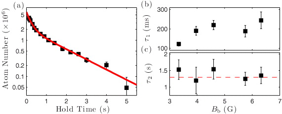To load the atoms into the ring trap the quadrupole coils are used in conjunction with an additional bias coil aligned along the -axis to raise the atoms in the quadrupole trap to overlap the cloud with the ring trap radius r_trap ~ 5 mm. Atoms are moved in 200 ms followed by a 10 ms hold time using a current ramp optimized to minimize heating, resulting in 1.1 × 10⁷ atoms in the quadrupole trap with a temperature of 40 μK and radius σ = 0.6 mm. The quadrupole trap is then turned off, and the ac drive coils and vertical bias field turned on. As a consequence of the coil geometry the quadrupole coils are strongly inductively coupled to the ac drive coils, and must be electrically isolated using an external relay that imposes a 0.5 ms delay between disabling the quadrupole and enabling the ac amplifier. The atoms then freely evolve in the ring trap for a variable time, before turning off the ring trap and performing absorption imaging of the atoms using a circularly polarized probe beam aligned along the -axis after a 3 ms time of flight. Due to the large and fluctuating Zeeman shift caused by the ac magnetic field amplitude it is not possible to image the atoms in the trap directly.

One of the challenges of using a single-chamber vacuum system for the ac ring trap arises due to copper acting as an efficient getter material for rubidium atoms. This leads to a build up of rubidium atoms on the ring from the background vapour required for loading the MOT. At the peak ac drive amplitude there is over 4 W of power dissipated in the ring, leading to a heating rate of 2 K s⁻¹. The effect of this heating for long trap hold times or over accumulated experimental runs is to release rubidium from the copper surface, leading to a significant enhancement of the rubidium vapour pressure and consequently reducing the background limited lifetime in the trap and leading to large shot-to-shot atom number fluctuations. The use of OFHC copper, with its inherently low vacuum outgassing rates [39], for the ring ensures that the increase in vapour pressure is primarily due to the release of adsorbed rubidium atoms.

This issue was circumvented using low rubidium vapour pressures and long (8 s) MOT load times, with regular cleaning cycles performed by running the ac field at full power for up to an hour and waiting for the vapour pressure to recover. This problem might be overcome using UV light to perform light assisted atomic desorption [40] to prevent a build up of atoms on the copper ring, or coating the ring using an insulating material such as sapphire which acts as a less efficient getter of Rb.

4. Results

The theoretical analysis of the time-averaged ring potential presented in section 2 reveals the importance of the position of the instantaneous magnetic field zeros during each cycle of the ac field to avoid violating the adiabaticity requirement. To characterize this effect, data are taken for a range of ac field amplitudes B₀, which determine the initial trap depth, and bias fields B_b that control the adiabaticity of the ring potential.

Figure 3 shows absorption images of atoms after 200 ms evolution in the ring trap at B₀ = 110 G for B_b = 4.6 G (b) and 9.2 G (c), with each image being the average of ten repeats. These demonstrate the time-averaged potential creates a large radius, cylindrically symmetric waveguide for cold atoms. The effect of the vertical bias on the trap is clearly visible, with the width measured from the standard deviation of the radial distribution changing from a thin ring of σ_r = 0.19 mm to a wide ring with σ_r = 0.51 mm as the B-field zeros are pushed further from the trap centre, as illustrated in figure 2(c). As discussed above, the instantaneous zeros cause hot atoms to be lost from the trap leading to a truncation of the radial velocity distribution. This is observed as an effective radial temperature of 7 ± 0.5 μK, measured from time of flight expansion of atoms released from the ring. However, due to the low density and trap frequencies the collision rate is too small to enable rethermalization within the ring, making this technique ineffective for evaporation as is done with the circle of death in a top trap [33]. The lack of thermalization can be seen from the cloud maintaining an azimuthal velocity distribution corresponding to the 40 μK of the initial quadrupole trap as it expands to fill the ring. Using a harmonic approximation for the bottom of the potential, the radial trap frequency can be estimated from the measured cloud size as , resulting in a trap frequency of 10 ± 1 Hz, comparable to the predicted frequency in figure 2(d). The relationship between the effective radial temperature and the lowest energy trap zero, T₀, is complicated due to the spatial selectivity of the field zeros, however both increase with the applied bias field due to increasing the energy scale over which the trap remains fully adiabatic. This is seen from the increase in the effective radial temperature to 18 ± 2 μK for the trap in figure 3(c). For higher bias fields, the anharmonicity of the trap precludes accurate measurement of the radial temperature and trap frequency as we are unable to observe the cloud for a sufficiently long time for the velocity distribution to dominate over the initial spatial distribution due to expansion of the cloud under the copper ring.

An additional consequence of the increasing bias field is a reduction in the axial trap frequency ω_z, leading to enhanced gravitational sag of −g/ω²_z. This reduces the trap radius from r_trap = 5.12 mm in (b) to 4.84 mm in (c), which can be understood from the contour plot in figure 2(d). A larger variation in radius is observed for smaller B₀ due to the reduction in the initial axial trap frequency. This behaviour shows good agreement with the finite element model discussed above for the trap parameters, enabling the atoms to be used as a probe of the magnetic field.

An important parameter in characterizing the trap geometry is the loading efficiency from the quadrupole trap, and hence atom number within the trap. Figure 4 shows the atom number after 200 ms in the ring as a function of drive field and applied bias. This timescale is chosen to enable the atoms to spread round and completely fill the ring and to enable any untrapped atoms to fall out of the field of view of the probe beam. The peak atom number loaded into the ring at B₀ = 66 G is 4.5 × 10⁶ corresponding to 43% of the initial number in the quadrupole trap, limited by the finite mode-matching between the quadrupole trap into the ring trap. Comparison of the required minimum bias field to the threshold value required to observe atoms in the ring trap shows good agreement with (2) above, which predicts B_b > 3 G for B₀ = 55 G.

Figure 4. Ring trap characterization of atom number in the ring trap after 200 ms as a function of applied bias field for different ac field amplitudes, B₀. Gaussian fits are shown as a guide to the eye, with errorbars equivalent to the markersize. Inset: scaled data showing universal scaling of ring parameters with ξ (see text).

The variation of atom number with the bias field displays an approximately Gaussian dependence. Qualitatively this trend can be understood from the scaling of the trap properties with bias field B_b, which linearly reduces the depth of the trap while linearly increasing the radial separation of the instantaneous zeros on either side of the minimum and pushing them to higher T₀. Initially, above the threshold value the increased separation of the zeros reduces the non-adiabatic losses, increasing the useful volume of the ring trap and enabling more atoms to be loaded from the MOT. For higher bias field the gain in radial width comes at the cost of a loss of trap depth and the hot cloud can no longer be loaded. Interestingly, we observe a phenomenological scaling of the peak atom number within the trap in terms of the parameter ξ = (B₀ − c)/(m × B_b) as illustrated in the inset of figure 4, where parameters m = 5.6 and c = 26 G are extracted from a straight line fit to the value B_b corresponding to the peak atom number as a function of B₀. The coefficients m and c give the scaling of bias field to drive field and the minimum ac amplitude required to obtain a ring trap respectively, with values of ξ = 1 corresponding to the optimum mode matching between the atomic distribution and the ring trap. The exact values of c,m are dependent upon the temperature of the initial atomic sample.

Analysis of the lifetime within the ring potential provides further evidence for this interpretation. Figure 5(a) shows atom number as a function of hold time for B₀ = 55 G and a bias field of 4.6 G, showing a double exponential decay in the loss of atoms from the ring. Fitting the data allows extraction of the initially rapid fast decay time τ₁, caused by non-adiabatic losses as hot atoms are evaporated out of the ring potential by the instantaneous zeros, and the longer timescale, τ₂, associated with losses due to background collisions. Figure 5(b) shows the change in τ₁ as a function of bias field, which initially increases from 120 to 220 ms as the bias field increases from 3 to 5 G, consistent with the predicted increase of T₀ from 10 to 20 μK. For smaller bias fields, the τ₁ relaxation is so fast that it cannot be measured as during the first 50 ms the small signal from the few atoms remaining in the trap is obscured by the absorption from falling atoms that have not been loaded into the ring, after which time there are no atoms remaining. There is no further gain for higher bias due to the relaxation of the trap which only slightly increases T₀. Importantly however, the background limited lifetime τ₂ plotted in figure 5(c) shows no dependence on the applied bias field, giving an average of τ₂ = 1.2 ± 0.2 s which matches the measured lifetime in the quadrupole trap. The biased ring trap therefore creates an adiabatic ring potential for cold atoms, permitting background limited lifetimes and hence long interaction times for atomic interferometry. Observation of the initial non-adiabatic loss is a direct consequence of the relatively hot thermal distribution loaded from the quadrupole trap.

Figure 5. Ring trap lifetime at B₀ = 55 G. (a) Atom number at B_z =  4.6 G versus hold time in the ring showing a two-component decay, with short timescale τ₁ due to non-adiabatic losses and slow decay τ₂ due to background collisions. (b) Lifetime τ₁ versus B_z plateaus around 220 ms as the trap is made adiabatic. (c) Background-limited lifetime τ₂ is independent of bias, with quadrupole lifetime indicated by dashed line.

In addition to considering how the atom number changes in the ring potential, it is also interesting to consider the evolution of the atomic distribution within the circular waveguide. For atoms loaded into a thin ring with a relatively weak bias field, as seen in figure 3(b), the Gaussian spatial distribution determined by the initial quadrupole trap spreads ballistically around the ring, taking 120 ms to completely fill the ring potential, which is determined by the 40 μK azimuthal temperature. At long times the azimuthal density distribution has a variation of 10%, independent of time. This corresponds to a potential difference of approximately 4 μK across the ring, consistent with a smooth trap tilted at an angle of 4 mrad. One of the proposed advantages of using ac currents for creating magnetic traps is to overcome issues of corrugation due to the electron motion in the conductor. Subtracting off the 4 mrad tilt, we observe no evidence of corrugations in the time-averaged potential at this energy scale, however a significantly colder atomic sample is required to probe the smoothness at the 100 nK level relevant to interferometry using quantum degenerate gases.

For the wide ring geometry, with increased values of B_b, the evolution in the ring is strongly dependent upon the initial loading position of the quadrupole trap and it is possible to induce radial or centre of mass oscillations for atoms in the ring trap due to the shallow potential. Another feature of the wide ring potential that can be exploited is the curvature of the central region seen from figure 2(a), which can be used to act as a beam splitter for the atomic cloud. Figure 6 shows the evolution for atoms loaded on the outer edge of the trap for B₀ = 55 G and B_b = 4.6 G. Each image is the average of ten repeats, which shows the cloud being accelerated into the ring centre due to the initial radial displacement and being split into two separate counter propagating clouds which overlap at 150 ms and then refocus at the initial loading position around 300 ms. Videos of the ring evolution for this data and for a weak bias field are provided in the supplementary data (available from stacks.iop.org/NJP/14/103047/mmedia). This example demonstrates the versatility of the ring trap and enables the cloud to explore a large region of the Mexican hat potential. For interferometric applications the initial splitting can be achieved using a coherent optical Bragg scattering [41] to reduce the centre of mass radial oscillations associated with this method, suppressing losses due to atoms exploring the non-adiabatic regions of the time-averaged potential.

Figure 6. Evolution in the ring for B₀ = 55 G and B_b = 4.6 G. Atoms loaded on the edge of the ring trap can be split into two counter-propagating wave-packets using the curvature of the toroidal potential that spread out to fill the ring. The small circular fringes are due to imperfections in the imaging system.

5. Outlook and conclusion

Characterization of the trap properties as a function of the ac drive field and applied bias show the importance of meeting the requirements for adiabaticity by removing the instantaneous B-field zeros from the minimum of the trap. This leads to increased loading efficiency and a vacuum-limited lifetime at long times for atoms in the ring trap. Our current setup is limited by the relatively high initial temperature of the atomic sample and the 1 s background lifetime corresponding to a pressure of 10⁻⁹ Torr. However, a reduced pressure and using a colder sample or quantum degenerate gas would permit operation at a lower bias field, which could be achieved using a double-cell vacuum chamber and cooling in a magnetic or optical trap. This makes it possible to create rings with a tight harmonic radial confinement with radial trap frequencies of approximately 100 Hz to define a waveguide suitable for atom interferometry offering a large integration time. An important source of heating in the trap is current noise from the ac amplifier, however it is possible to reduce this to 1 part in 10⁵ using active feedback [42]. Our current ring has an area of A = 80 mm², leading to a rotation sensitivity of  [20] for a BEC of N = 10⁵ atoms in a single revolution. Extension to exploit the ring trap in this regime is the subject of further work.

We have presented the first demonstration of an inductively coupled ring trap for cold atoms which provides a viable technique for generating macroscopic toroidal waveguides for cold atoms. The main advantage over alternative approaches using current-carrying wires is that the trap potential is determined by the geometry of the conducting ring which can be machined to high tolerance, making it easy to define an axially symmetric trap without any end effects or distortions from the external coils.

Acknowledgments

This work has been supported by the EPSRC under grant EP/G026068/1. PFG received

Content from this work may be used under the terms of the Creative Commons Attribution-NonCommercial-ShareAlike 3.0 licence. Any further distribution of this work must maintain attribution to the author(s) and the title of the work, journal citation and DOI.

J D Pritchard et al 2012 New J. Phys. 14 103047
doi:10.1088/1367-2630/14/10/103047
© IOP Publishing and Deutsche Physikalische Gesellschaft
Received 18 July 2012
Published 30 October 2012

Related articles

• The Primer Fields #1 (Transcript) (thesingularityeffect.wordpress.com)
• Astronomers finally crack mystery of solar system’s strange ‘ribbon of energy’ – The Space Reporter (thespacereporter.com)

 

Think Magnetism 3 DRAFT

If the Aurora is a Magnetic field, then, we should think of them as being made up of  little  balls of energy.  Or, “Particles.” connected together.

That should be easy enough since that’s what we’re taught. Right?

(Well it should be .)

Anyway…, they’ve got to be really small, and they’ve got to be connected. So lets make them a shape that can touch,  (We already know that conduction allows for information (Ie. Energy) to be transmitted this way.) So something round.

Since they are (or will be) comprised of something, (particles) they therefore have mass.

So, we’ll give them each a field.  Call them Magnetic North and Magnetic South.

Kind of like the Earth.

And then apply this thinking now to “ALL”particles of Matter.

Even light.

Now, at this point, I have to remind you of something that theoretical physicist Mr. Richard Feynman once said.

Although he was literally correct in his assumption, it only served to hinder us in our understandings of what matter and energy are.  His assertion at the time, was based on the incorrect or unfinished definition of matter.

MATTER:   …”material substance that occupies space, has mass, and is composed predominantly of atoms consisting of protons, neutrons, and electrons, that constitutes the observable universe, and that is nonconvertible with energy.”

So let’s start here.

Ooops! I see one thing wrong already. There’s something missing from our definition.

It’s missing two key words  that have helped create common misunderstandings  in today’s understanding of matter. These words are “volume” and “Mass.”

When Mr. Feynman was speaking, he was referring to the fact that certain forms of energy did not posses these attributes at “rest,” and therefore were not considered “Matter.”

…”material substance that occupies space.” Well, We know it meets this requirement, because we  can observe it.  If it wasn’t “made of something, we couldn’t interact with it. Focus it, reflect it, store it, or generate it.

…”has mass,”  The thinking that caused Mr. Feynman to make his assertion, was that since they could not “ever” slow energy down to a “fixed” position like other pieces of matter, and that”solid matter”  did not move on its own volition,  or “emit” other forms of energy, that it must not fit into the same class.

…”is composed predominantly of atoms consisting of protons, neutrons, and electrons,“  This statement violates both previous assertions. But, we’ll give it credit anyway. …”
Now it is going to get a little complicated as we start discussing how these magnetic fields overlap each other and interact with each other.
Here we have the photon and its fields again.

We need to realize though that  in reality the electromagnetic fields do not just stop at the limits of the fields show here. They continue out much further, but they also get much weaker as they go further away from the photon.  But for now, let’s look at how the field develops.

The fields are attracted to this point where it passes between fields polarity barrier (See interference), one at a time, simultaneously  “reversing.” the particles polarity.

The flip point.

Showing the structure formation

 

 

 

Each one has an unlimited source (until all matter is absorbed) coming in, and  “jets” where excess energy is released.

Note the Horizontal “spin?”

Note how the field is created in vacuum with plasma?

 

 

See how energy forms?

Now, using this

 

 

Related articles

• Magnetism – Molder of the Universe (thesingularityeffect.wordpress.com)
• More Vindication (thesingularityeffect.wordpress.com)
• The Primer Fields #1 (Transcript) (thesingularityeffect.wordpress.com)

Let’s see if I’ve got this right

…”The size of the waveform is equal to the mass and the energy of the particle.”

I wonder if I just wrote my first law?

That would be so cool!

thesingularityeffect.wordpress.com

More vindication

NASA Discovers Hidden Portals In Earth’s Magnetic Field

Arjun March 8, 2013

http://www.collective-evolution.com/2013/03/08/nasa-discovers-hidden-portals-in-earths-magnetic-field/

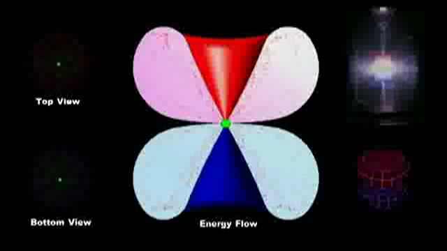
Our planet has come a long way in scientific breakthroughs and discoveries. Mainstream science is beginning to discover new concepts of reality that have the potential to change our perception about our planet and the extraterrestrial environment that surrounds it forever. Star gates, wormholes, and portals have been the subject of conspiracy theories and theoretical physics for decades, but that is all coming to an end as we continue to grow in our understanding about the true nature of our reality.

In physics, a wormhole was a hypothetical feature of space time that would be a shortcut through space-time. We often wonder how extraterrestrials could travel so far and this could be one of many explanations. Although scientists still don’t really understand what they have found, it does open the mind to many possibilities.

Turning science fiction into science fact seems to happen quite often these days and NASA did it by announcing the discovery of hidden portals in Earth’s magnetic field.  NASA calls them X-points or electron diffusion regions. They are places where the magnetic field of Earth connects to the magnetic field of the Sun, which in turn creates an uninterrupted path leading from our own planet to the sun’s atmosphere which is 93 million miles away.

NASA used its THEMIS spacecraft, as well as a European Cluster probe, to examine this phenomenon. They found that these portals open and close dozens of times each day. It’s funny, because there is a lot of evidence that points toward the sun being a giant star gate for the ‘gods’ to pass back and forth from other dimensions and universes. The portals that NASA has discovered are usually located tens of thousands of kilometres from Earth and most of them are short-lived; others are giant, vast and sustained.

As far as scientists can determine, these portals aid in the transfer of tons of magnetically charged particles that flow from the Sun causing the northern and southerns lights and geomagnetic storms. They aid in the transfer of the magnetic field from the Sun to the Earth. In 2014, the U.S. space agency will launch a new mission called Magnetospheric Multi scale Mission (MMS) which will include four spacecraft that will circle the Earth to locate and then study these portals. They are located where the Earth and the Sun’s magnetic fields connect and where the unexplained portals are formed.

NASA funded the University of Iowa for this study, and they are still unclear as to what these portals are. All they have done is observed charged particles flowing through them that cause electro-magnetic phenomenon in Earth’s atmosphere.

Magnetic portals are invisible, unstable and elusive. they open and close without warming and there are no signposts to guide is in – Dr Scudder, University of Iowa

Mainstream science continues to grow further, but I often get confused between mainstream science, and science that is formed in the black budget world. It seems that information and discovery isn’t information and discovery without the type of ‘proof’ that the human race requires. Given that the human race requires, and has a certain criteria for ‘proof’, which has been taught to us by the academic world, information can easily be suppressed by concealing that ‘proof’. It’s no secret that the department of defence receives trillions of dollars that go unaccounted for and everything developed within the United States Air Force Space Agency remains classified. They are able to classify information for the sake of ‘national security’. Within the past few years, proof has been emerging for a number of phenomenon that would suggest a whole other scientific world that operates separately from mainstream science.

We have the technology to take ET home, anything you can imagine we already have the technology to do, but these technologies are locked up in black budget projects. It would take an act of God to ever get them out to benefit humanity – Ben Rich, Fmr CEO of LockHeed Skunk Works

I use this video a lot in many of my posts, but it is just a profound statement, I love to use it over and over. He is x NASA personnel so it kind of fits in with the article.

Sources:

http://science.nasa.gov/science-news/science-at-nasa/2012/29jun_hiddenportals/

http://www.nasa.gov/mission_pages/sunearth/news/mag-portals.html

As stuff breaks

Never ending liht bulbs?

 Dynamical Casimir effect in meta material converts vacuum fluctuations into real photons

phys.org

(Phys.org) —In the strange world of quantum mechanics, the vacuum state (sometimes referred to as the quantum vacuum, simply as the vacuum) is a quantum system’s lowest possible energy state. While not containing physical particles, neither is it an empty void: Rather, the quantum vacuum contains …..

 

• 

  St**** So**rF**:

  I can show you a video of it.

  It’s another (3 now I think) covered within the Primer Fields that Azure brought to my attention in Ray‘s group.

  Oh, and I meant the technical papers released “SINCE” the video…:)
• 

  M*** M**the:

  wow!.. where is the Video? thanks
• 

  St**** So**rF**:

  Start here,

  The Primer Fields Part 1

  In this video series the currently accepted theories of physics and astrophysics…See More
• 

  D** R2D2:

  In the first several minutes of that video I’m already highly skeptical of the scientific merit. He doesn’t speak like a scientist at all. Scientists have hypothesis, this guy says unequivocally that he has the answer.
  
  I don’t have the domain expertise to claim he’s wrong on a factual basis but judging by the way he speaks I doubt there’s much to his claims.
• 

  St**** So**rF**:

  I would say keep watching. As to the voice, I assume it’s an actor. As to the assertion? How else do you attack an accepted theory. I have been informed that the thesis has been submitted to a number of journals, but no specifics. I have checked the re…See More
• 

  St**** So**rF**:

  I know that all sounds truncated, I’ll try to clarify….”I could fin…” In this statement, I mean, I couldn’t find anyone conducting and publishing results in the field, nor has anyone even suggested it. BUT..If you look at the work that HAS been pub…See More
• 

  St**** So**rF**:

  Sorry again. Third journal publication: http://phys.org/news/2013-03-nihilo-dynamical-casimir-effect-metamaterial.html – https://thesingularityeffect.wordpress.com/2013/03/03/some-vindication/ – Still looking for the other one

  
• 

  St**** So**rF**:

  This just popped up on Kurzweil in between posts.

  NASA Discovers Hidden Portals In Earth’s Magnetic Field

  Our planet has come a long way in scientific breakthroughs and discoveries. Main…See More

Related articles

• What I Think – The Primer Fields (thesingularityeffect.wordpress.com)
• Ex nihilo: Dynamical Casimir effect in metamaterial converts vacuum fluctuations into real photons (phys.org)

 

Isn’t it funny…?

Isn’t it funny…?

 

…”How, as soon as they discovered the Higgs Boson…

They realized that it destroyed the model!

                                                                                                                                         Richard Brown

Some Vindication

Getting around the ‘uncertainty principle’: Physicists make first direct measurements of polarization states of light

 Physicists make first direct measurements of polarization states of light March 3, 2013 Getting around the Uncertainty Principle Enlarge Weak measurement: as light goes through a birefringent crystal the horizontally and vertically polarized components of light spread out in space, but an overlap between the two components remains when they emerge. In a “strong” measurement the two components would be fully separated. Credit: Credit: Jonathan Leach Researchers at the University of Rochester and the University of Ottawa have applied a recently developed technique to directly measure for the first time the polarization states of light. Their work both overcomes some important challenges of Heisenberg’s famous Uncertainty Principle and also is applicable to qubits, the building blocks of quantum information theory. Ads by Google Medical Billing Software – Watch the ADP AdvancedMD Billing Software Video Demo Online Now – ADP.AdvancedMD.com/Billing-Software They report their results in a paper published this week in Nature Photonics. The direct measurement technique was first developed in 2011 by scientists at the National Research Council, Canada, to measure the wave function – a way of determining the state of a quantum system. Such direct measurements of the wave function had long seemed impossible because of a key tenet of the uncertainty principle – the idea that certain properties of a quantum system could be known only poorly if certain other related properties were known with precision. The ability to make these measurements directly challenges the idea that full understanding of a quantum system could never come from direct observation. The Rochester/Ottawa researchers, led by Robert Boyd, who has appointments at both universities, measured the polarization states of light – the directions in which the electric and magnetic fields of the light oscillate. Their key result, like that of the team that pioneered direct measurement, is that it is possible to measure key related variables, known as “conjugate” variables, of a quantum particle or state directly. The polarization states of light can be used to encode information, which is why they can be the basis of qubits in quantum information applications. “The ability to perform direct measurement of the quantum wave function has important future implications for quantum information science,” explained Boyd, Canada Excellence Research Chair in Quantum Nonlinear Optics at the University of Ottawa and Professor of Optics and Physics at the University of Rochester. “Ongoing work in our group involves applying this technique to other systems, for example, measuring the form of a “mixed” (as opposed to a pure) quantum state.” Previously, a technique called quantum tomography has allowed researchers to measure the information contained in these quantum states, but only indirectly. Quantum tomography requires intensive post-processing of the data, and this is a time-consuming process that is not required in the direct measurement technique. Thus, in principle, the new technique provides the same information as quantum tomography but in significantly less time. “The key to characterizing any quantum system is gathering information about conjugate variables,” said co-author Jonathan Leach, who is now a lecturer at Heriot-Watt University, UK. “The reason it wasn’t thought possible to measure two conjugate variables directly was because measuring one would destroy the wave function before the other one could be measured.” The direct measurement technique employs a “trick” to measure the first property in such a way that the system is not disturbed significantly and information about the second property can still be obtained. This careful measurement relies on the “weak measurement” of the first property followed by a “strong measurement” of the second property. First described 25 years ago, weak measurement requires that the coupling between the system and what is used to measure it be, as its name suggests, “weak”, which means that the system is barely disturbed in the measurement process. The downside of this type of measurement is that a single measurement only provides a small amount of information, and to get an accurate readout, the process has to be repeated multiple times and the average taken. Boyd and his colleagues used the position and momentum of the light as the indicator of the polarization state. To couple the polarization to the spatial degree of freedom they used birefringent crystals: when light goes through such a crystal, there is a spatial separation introduced for different polarizations. For example, if light is made of a combination of horizontally and vertically polarized component, the positions of the individual components will spread out when it goes through the crystal according to its polarization. The thickness of the crystal can control the strength of the measurement, weak or strong, and determine the degree of separation, correspondingly small or large. In this experiment, Boyd and his colleagues passed polarized light through two crystals of differing thicknesses: the first, a very thin crystal that “weakly” measures the horizontal and vertical polarization state; the second, a much thicker crystal that “strongly” measures the diagonal and anti-diagonal polarization state. As the first measurement was performed weakly, the system is not significantly disturbed, and therefore, information gained from the second measurement was still valid. This process is repeated several times to build up accurate statistics. Putting all of this together gives a full, direct characterization of the polarization states of the light

A quoteable quote

     …” Some of you are really starting to get it. Gravity is not a force unto itself. It is a manifestation of EM forces. Who knows where this will all lead. Meet George Jetson!…”                                                                                                                      David LaPoint

Neodymium magnet in FAT copper pipe

 

Sage advice wise one…But to do that I would first have to learn control..

The Primer Fields

thesingularityeffect.wordpress.com

Magnetism—Molder of the Universe

http://plasmauniverse.info/mag_fields.html

The Atlas as it has been realized in the following pages illustrates again that galaxies cannot be characterized as just assemblages of stars, radiation, and gravitation. The following Atlas pictures emphasize the importance of dust in some; they particularly imply a much more important role for the gas in general and point to the existence of either new forces or forces which previously have been little considered. For example, the twisted, distorted shapes and curious linkages pictured here attest to the fact that there are viscocity-like forces present that in some cases are dominant. Probably these forces are due to magnetic effects. Vorontsov-Velyminov has stressed in the past the probable magnetic nature of these effects. Magnetic forces are very difficult to study, but may be very important in our Universe. The recent radio-astronomy discoveries of violent events in galaxies reveal sources of energetic charged particles. These charged particles interact with magnetic fields and offer the hope of mapping, measuring, and understanding cosmic magnetic fields. Exploration of the connection between the plasmas observed with the radio telescope and the optical evidences of plasma effects picture in the present Atlas in now open to us.

Halton Arp, Atlas of Peculiar Galaxies, University of Chicago Press, Chicago, Illinois, 1966.
Helicity and Filamentation, the Signature of a Magnetic Field. The data shown is on the extragalactic, or cosmic, scale.

Magnetism is the fundamental force that determines the character, or motion or shape of ionized matter (plasma). The degree of ionization in interplanetary space and in other cosmic plasmas may vary over a wide range, from fully ionized to degrees of ionization of only a fraction of a percent.\footnote{The degree of ionization is defined as $n_p/ \left( {n_0+n_p} \right)$ where $n_p$ is the plasma density and $n_0$ is the density of neutral particles.} Even weakly ionized plasma reacts strongly to electromagnetic fields since the ratio of the electromagnetic force to the gravitational force is 39 orders of magnitude. For example, although the solar photospheric plasma has a degree of ionization as low as 10$^{-4}$, the major part of the condensable components is still largely ionized. The “neutral” hydrogen (HI) regions around galaxies are also plasmas, although the degree of ionization is only 10$^{-4}$. Most of our knowledge about electromagnetic waves in plasmas derives from laboratory plasma experiments where the gases used have a low degree of ionization, 10$^{-2}$-10$^{-6}$.

Because electromagnetic fields play such an important role in the electrodynamics of plasmas, and because the dynamics of plasmas are often the sources of electromagnetic fields, it is desirable to determine where within the universe a plasma approach is necessary. Of primary importance is the magnetic field. On earth, magnetic field strengths can be found from about 0.5 gauss ($0.5 \times 10^{-4}$ T) to $10^7$ gauss ($10^3$ T) in pulsed-power experiments; the outer planets have magnetic fields reaching many gauss, while the magnetic fields of stars are 30-40 kG (3-4 T). Large scale magnetic fields have also been discovered in distant cosmic objects. The center of the Galaxy has milligauss magnetic field strengths stretching 60 pc in length. Similar strengths are inferred from polarization measurements of radiation recorded for double radio galaxies. No rotating object in the universe, that is devoid of a magnetic field, is known.

In cosmic problems involving planetary, interplanetary, interstellar, galactic, and extragalactic phenomena, magnetohydrodynamics effects are appreciable. Neglecting lightning, planetary atmospheres and hydrospheres are the only domains in the universe where a nonhydromagnetic treatment of fluid dynamic problems is justified.
The Helix Nebula

Effects of a Magnetic Field

The most basic difference between ionized and nonionized matter is the ability to carry electric current. This ability is also the reason why virtually all the matter in the universe is—and presumably has always been—magnetized. The presence of the magnetic field has important dynamical consequences since the magnetic force can locally be much greater than the gravitational force.

The ability of carrying current, which is the basis for the magnetization, is a property that is still not well known in the case of cosmical plasma. It can be different by many powers of ten from what classical theories predict.

In laboratory and space plasma electric currents tend to cause filamentation. Filamentary structures are also abundant in the cosmical plasma and make homogeneous models of astrophysical plasma very dubious. Correspondingly, homogeneous models are likely to be misleading when applied to large-scale astrophysical processes.

One of the notable characteristics of space plasma, revealed by satellites and space probes, is its tendency to form sharp boundaries between plasmas with different properties. This tendency towards “cellular structure” can have profound astrophysical implications such as generating electric fields in space and providing sources of energy for driving electric currents over very large distances.

A phenomenon called critical ionization velocity, first proposed in Alfven’s cosmogonic theory, has been observed in both laboratory and space plasmas. It implies, among other things, an exchange of momentum between plasma and neutral gases in the presence of magnetic fields. One of the surprising discoveries in the near-Earth plasma is the existence of previously unknown mechanisms that allow very efficient separation of different chemical species. Even more surprisingly, is the recent discovery through radiotelescope observations that interstellar space displays the same phenomena.
The Magnetized Plasma

Plasma, which is rare in our close environment, is the dominating state in the universe as a whole. The Sun and stars as well as the diffuse matter between them and between the galaxies are all in this state, despite their great difference in density and temperature. The only exceptions are the cold celestial bodies such as the Earth and other planets, the satellites, asteroids, comets, meteoroids, and dust grains, all of which account for an extremely small fraction of the know matter in the universe. Furthermore, all the cosmical plasma is magnetized. From the nearest cosmical plasma—the Earth’s ionosphere—out to the most distant intergalactic regions all cosmical plasma are penetrated by magnetic fields that influence their physical properties in various, often dramatic, ways.

In diffuse matter, which forms a major part of the universe, the motion of each individual particle is strongly controlled by the magnetic field. For example, a hydrogen ion in the solar wind with a thermal velocity of 20 kilometers per second in the interplanetary magnetic field of 5 nanotesla experiences a magnetic force of that is about 10^7 times stronger than the gravitational force from the Sun. Even in the other extreme, for example, in stellar interiors, where gravitational forces dominate, the magnetic field makes possible wave modes (such as Alfvén waves) that are not possible in nonionized media.

Except in very limited circumstances, all cosmical plasmas carry electric currents that constitute the sources of the magnetic field.

Contours of ‘neutral’ hydrogen regions superposed on an optical image of the galaxy NGC 4151. The Contours show two hydrogenic plasma density ‘peaks’ (left and right) situated about a void at the center of the galaxy.

Magnetic field derived from galaxy simulation overlaid on the galaxy NGC 4151. The blue ‘ribbons’ are components of a vertical magnetic field while the green arrows depict both the axisymmetric and bisymmetric magnetic fields observed in galaxies of this morphological type.

Left: Simulation magnetic energy density superimposed on simulation galaxy. A ‘horse-shoe’ shaped cusp, opening towards a spiral arm surrounds a magnetic field field/HI minima core.

Right: HI distribution superimposed on an optical photograph of the galaxy NGC 4151.

Intergalactic Magnetic Fields

One of the most compelling pieces of evidence for the existence of supercluster-sized Birkeland currents came from the discovery of faint supercluster-scale radio emission at 326 MHz between the Coma cluster of galaxies and the Abell 1367 cluster. The radiation’s synchrotron origin implies magnetic field strengths of 0.3-0.6 microgauss stretching for 1.5 megaparsecs. This corresponds to a classical galactic Birkeland current of nearly 10^19 amperes.
Conclusions

The photographs in the Atlas of Peculiar Galaxies are completely familiar to high energy density plasma experimentalists For example, the physicist Winston Bostick could sequence the photographs in the Atlas according to type and time evolution, based on his observation of millimeter sized colliding plasmas in pulsed power generators. The shapes are, indeed, dependent on the magnetic field as can be demonstrated in three-dimensional electromagnetic-gravitation particle-in-cell simulations.